PyVWF: bias-corrected wind power from reanalysis

A uniform correction treats reanalysis bias as one number. It is not. It varies by region, by season and by the terrain a turbine sits in, so a single scaling factor fixes the national average and leaves the local errors in place.

• A Python rewrite of Iain Staffell's Virtual Wind Farm model, which underpins the wind simulations on Renewables.ninja, implementing the granular method from my 2024 Energy paper.
• Turbines are clustered spatially and their generation grouped in time. A scalar and an offset are fitted per cluster and period against observed generation, then applied to ERA5 wind speeds.
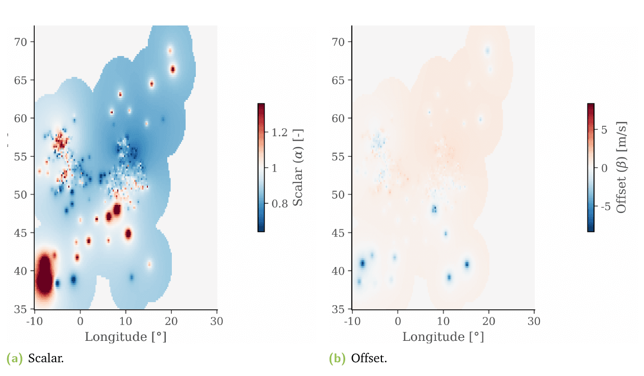
• Correction factors from control points are interpolated onto the native ERA5 0.25° grid. Four interpolation methods were compared under spatial cross-validation; inverse distance weighting was chosen for bounded extrapolation and stability where control points are unevenly spread.
• Observed generation is sourced and vetted per country, from individual turbines up to whole countries: ENTSO-E, AEMO, CAMMESA, CEN, EIA, EMI, ONS and UK sources, with registries such as the Marktstammdatenregister and REPD for turbine metadata.

• Denmark, 76 correction configurations: intermediate spatial resolution with seasonal or bimonthly grouping generalised best, and over-fitting at high resolution was measured with elbow and silhouette diagnostics rather than assumed.
• Energy (2024): trained on 3,389 Danish onshore turbines over 2015 to 2019, validated on 2020 with 4,834 turbines, 1,445 of them new, so the test was independent in both time and space.
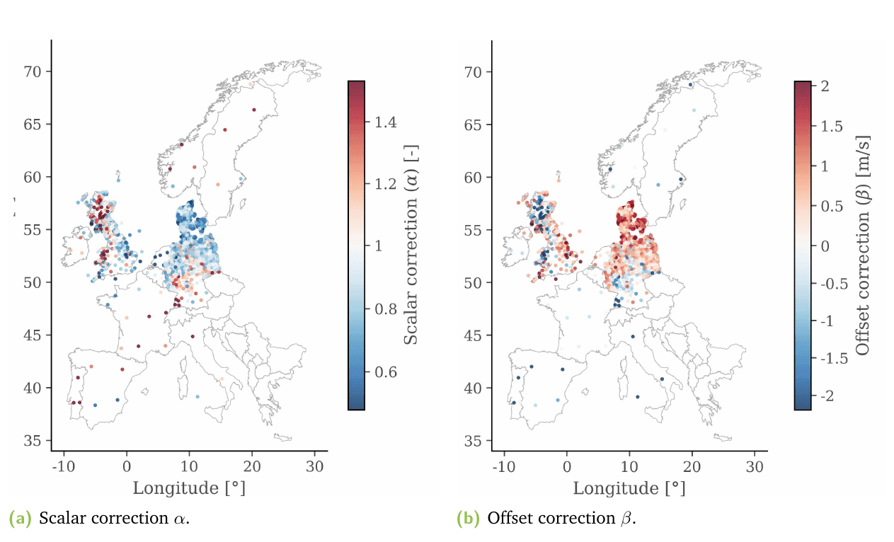
• Europe: corrections from 1,729 control points in 12 countries, gridded over 23,989 ERA5 cells (161 × 149), reduced capacity-factor MAE by 16 to 79% against uncorrected ERA5.
• Borrowing information across Europe outperformed country-specific corrections in several countries.
• Regions where observation density could not support a reliable value were masked rather than published as part of one unqualified surface.

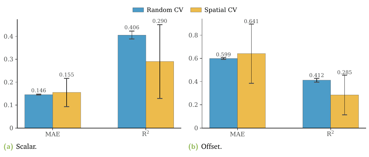
• Terrain-informed machine learning, 27 features across 23,009 turbines in Denmark, the UK and Germany. Random cross-validation gave R² of 0.35 to 0.41. Nearby turbines share weather, so those folds were not independent.
• Under spatial cross-validation the ranking changed: Elastic Net 0.295, Ridge 0.293, random forest 0.271, gradient boosting 0.261. Holding out the UK, the random forest fell to −0.376 and Ridge was the only model above zero.
• I reported the lower figures and kept geometric interpolation as the published method. A feature ablation showed ERA5's own wind climatology carries most of the predictable signal; turbine and land-cover features added almost nothing.
• Norway's hourly per-plant file turned out to be modelled rather than measured, so Norway is not used as a validation fold.

• I wrote all 310 commits in the v0.5.1 release, published with a Zenodo DOI.
• 469 test functions across 44 files in that release; CI on a Python 3.10 to 3.12 matrix with ruff and mypy enforced, PEP 561 typing, and Sphinx docs built with warnings as errors.
• Docker exercised in CI, every example script executed in CI, import-linter layer contracts, pre-commit, Dependabot and semantic versioning.
• The validation scorecard is re-run end to end from one commit on a clean tree. Every run manifest records the commit, whether the tree was dirty, and library versions. Superseded results are kept with dated correction notices, not deleted.
• The scorecard flags its own weak rows: 7 of 9 turbine-level rows rest on at least one degenerate fit, and only Denmark and New Zealand are clean.
• Refactored and extended with Claude Code from early 2026, on top of the pre-2026 research code.

PyVWF became a package when MSc and PhD students started projects on top of it. When a PhD student could not get their own data into the model, I wrote a documented input framework with an example notebook. They got their data working, and I used the same pipeline to integrate much more data myself.

Energy system models plan decades of investment on wind inputs that are rarely questioned. I extended PyPSA-Eur to test how much three of those inputs, reanalysis bias, wake losses and spatial resolution, change the answer.

Bias corrections only exist where there is observed generation to learn from. This work asks whether a constrained, physics-informed model can carry a correction to a region it has never seen, and fixes the tests before running them.